PID theory: Multiple time constants

In the previous section we looked at a simple dynamic system, a thermometer, and developed the concept of a the time constant, being how long it takes for 62.3% of any change to appear in the output. What about a more complex system, like our initial heater, water and thermometer?

It turns out that systems may have, and very often do have, multiple time constants that are cascaded. That means the output of one time constant element drives the input of another. In the electric kettle experiment there are probably at least 3: The heating element, the water and the thermometer.

Let's see what we can expect out of such a system if we apply a step change to its input (by step change we mean we apply a certain level of power (or whatever) and hold it constant) while we observe the output.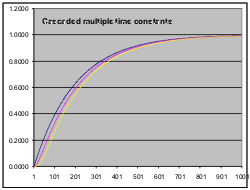

The spreadsheet "multipleTC.xls" lets you explore multiple time constants. (This spreadsheet contains macro code, but it is quite harmless ... trust me!)

multipleTC.xls has three cascaded time constants, represented by the columns Stage 1, Stage 2 and Stage 3. The "input" to each column is the column to its immediate left. Hence, the input to Stage 1 is a column full of 1's. We call this a "unity step input". You can toggle the input to become 1's for half the time and 0's for the rest, using the "Input" button. More on that later ... (if you are using OpenOffice, the Input button won't work. Move it aside and instead alternate the contents of cell H3 between 1 and 0. Beware: OpenOffice is very slow, so you may not see a result for a few seconds. Also, the curves will be in different colours that do not key to the column headings.)

Above each column is a constant 'K'. This controls the effective time constant for that column. The higher K, the shorter the time constant. If you set K=1 you effectively bypass that stage. If you set K=0 you create an infinite time constant, and the output will never change.

The formula for each new value is

New_Value = Old_Value * (1-K) + Input * K

Basically this equation says the following: Suppose K is 0.1. Then for each new input reading, we produce a new output that consists of 10% of (K times) the new input plus 90% of (1-K times) the old output. That means that if the input changes we don't pass the whole change to the output right away. The smaller K is the longer it will take the output to catch up with the input.

The 3 stages are plotted in blue for the 1st stage output, magenta for the 2nd stage output and yellow for the 3rd stage output. The input is plotted in turquoise. You can change the input with the "Input" button.

The initial K values are 0.005, 0.05 and 0.05. If you look down the Stage 1 column for a value of 0.632 (the "magical" 1 time-constant value) you will find the closest value at row 200. It just happens that 200 is 1/K for that column.

For time constants much greater than the sampling interval, K is approximately Tau/Ts (Ts being the sampling time). A better formula is

K = 1 - Exp( -Ts / Tau)

This gives the right answers for all time constants. Remember however that a sampled system is an approximate representation of a continuous process, and it will get worse the longer Ts is relative to Tau.

Take a look now at the very start of the graph. Make sure the K values are set back to their original settings if you have been playing with them. The yellow curve (Stage 3) seems to start slowly and then accelerate. There's an initial hesitation before it gets going. That was exactly what happened with the electric kettle when we first applied the power! In fact, at first we couldn't see any change at all.

Imagine what the means for our poor controller. It applies a control input to the process, and at first nothing seems to happen at all. Without going into too much theory, the more cascaded time constants a process contains, the harder it will be to a control. What's more the closer together the slowest of those time constants are, the worse it will be. We call the slowest time constant the "dominant time constant". If the dominant time constant is say 10 minutes and the next slowest one is 1 second, we can probably ignore all but the dominant one. If the next slowest time constant is 9 minutes, we are more likely to have trouble.

Let's now look at what happens when the input turns off. Click the "Input" button. This makes the input turn off at the half-way point across the graph. You should immediately notice that the yellow output continues to rise after the input goes away. There's the cause of the overshoot we had with the kettle! (Remember in the first run with the kettle, we turned off the power at 80ºC but the temperature coasted up to 87ºC?). Try changing the K factors for stages 2 and 3. With values closer to K for stage 1 the relative overshoot can become quite severe.