PID characterization: Extracting the time constants
Now we come to the fun part, and the part that will determine the eventual success of the whole exercise: Establishing the time constant(s) of your process. This is where your Excel skills come into play.
In the spreadsheets folder you will find a file called "Rising analysis.xls". Make a copy and load that file into Excel now. The first few rows are reproduced below. This is the actual data I acquired from my contraption. Our objective is to establish the 3 time constants in the top row (Tau). We will start with a practice run using my data.
| A | B | C | D | E | |
|---|---|---|---|---|---|
| 1 | Tau | 450 | 50 | 150 | |
| 2 | K | 0.0018 | 0.0100 | 0.0132 | |
| 3 | |||||
| 4 | Raw | Normalised | TC1 | TC2 | TC3 |
| 5 | 0.19608 | 0.00000 | 0.00000 | 0.00000 | 0.00000 |
| 6 | 0.19608 | 0.00000 | 0.00222 | 0.00002 | 0.00000 |
| 7 | 0.19608 | ||||
| 8 | 0.19608 | ||||
| 9 | 0.19608 |
The first data column is the raw data. It starts at 0.196 and rises to a final value of 0.549 way down the sheet. You will eventually be pasting your data into this column. Because you will have a different number of data points, you will have to reconstruct the other columns. That is why I've left all but the first two rows blank.
Highlight the last 4 cells of data in row 6 (the 2nd data row), i.e. the range C6:E6 and copy it (CTRL+C). Now highlight every cell in column B from B7 down to the last row of raw data, then paste (CTRL+V). This should give you a fully filled in table with 5 columns of data down to row 3514. In doing this you have replicated the formulas for the normalised data and the 3 time constants. The normalised data is just the raw data offset and re-scaled to the range 0-1.

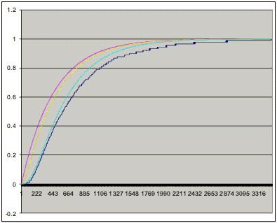
Now highlight all the data in columns B through E and do a line chart. It should look like the one reproduced here.
What you have here is the original data as a jaggedy black graph plus the 3 time constant "outputs" in magenta, yellow and cyan.
You now have to manipulate the 3 time constant numbers so one of the graphs overlays the original data as closely as possible. That is an art, not a science, so you are kind of on your own here! Just experiment with the numbers until you get the hang of it.
One trick I have discovered is to approximate the dominant time constant as follows:
- Locate the row in column B where the value is close to 0.2
- Locate the row in column B where the value is close to 0.7
- Calculate the time difference between the two points. This is a good first approximation to Tau1 (cell C1)
Note: If your process is inverting, i.e. its output decreases as the control input increases, swap the names on the template Excel files before you start. In my nomenclature "rising/increasing" and "falling/decreasing" refer to the process input, not its output.
Once you have developed an understanding of how the spreadsheet works, load in your own data. The best way is to make and rename a copy of my file, then delete my raw data from column A. Then load your log file *.csv into Excel, copy and paste column 1 into the new spreadsheet. Click on cell B6 and look at its formula. You will see a reference to cell $A$3514. That was the very bottom cell of my data. When you have your data pasted in you will have to change that reference to the last cell of your data and then re-build columns B through E as outlined above. Now fiddle around to find the time constants.
The exercise so far gives you a set of time constants for rising output. In most cases this applies also to falling outputs. Only in rare and special cases will the rising and falling responses be different. If you have very good reason to believe your process is asymmetrical then repeat the exercise for a falling output.
There is a spreadsheet "Falling analysis.xls" to help you. Delete my data from row 7 down and paste in you data. The process is exactly the same as before. I've "flipped" the data so that even though the output is falling it appears as rising on the graph. I simply found it easier to visualise that way round.
You should now have one or two sets of time constants, one for rising output and possibly one for falling output. Note the time constants and save your spreadsheets. If you have a symmetrical process you will use the same set of time constants for rising and falling.
By the way, going for 3 time constants and not 2, or 5 or 11, is somewhat arbitrary. My experience is that you can get a fairly decent match to the process with 3, and PIDassist supports 3.
